Deriving Actor-Critic method along with some intuition

Posted on 28^th October, 2023

Pre-requisite: Basics of Reinforcement Learning (RL)

Please feel free to skip any of the content if you know it aprior

Content:

• Introduction
• Classification of reinforcement learning methods
• Monte-Carlo Policy-Gradient Method (REINFORCE)
• Variance reduction technique
• Policy gradient with reward-to-go
• No-Bias proof
• Variance reduction proof
• Policy gradient with baseline
• No-Bias proof
• Baseline derivation for least variance
• Actor-Critic Method

Introduction

In reinforcement learning, Agent interacts with the environment to learn a policy. This policy can be represented as \(\pi_{\theta}\) parameterized by \(\theta\) which is a distribution over action for a given state i.e \(a \sim \pi_{\theta}(s)\). The policy usually is represented by \(\pi\) as it is stochastic in nature, this stochasticity makes the agent capable of exploring the environment. We need to know few notations: \begin{align*} s_i & \leftarrow \text{state of the agent at }i^{\text{th}}\text{ timestep}\\ a_i & \leftarrow \text{action taken by the agent based on }s_i\\ r_i & \leftarrow \text{reward at }i^{\text{th}}\text{ timestep} \\ \tau & \leftarrow s_0,a_0,s_1,a_1,s_2,....s_T\\ R(\tau) & \leftarrow \text{total reward} \\ s' & \leftarrow \text{next state}\\ s_T & \leftarrow \text{terminal state} \end{align*} where \(r_i=f(s_i,a_i,s_{i+1})\)
As the policy is probabilistic in nature, so the trajectory/path(\(s_0,a_0,r_0,s_1,a_1,r_1,s_2,....s_T\)) followed by the agent is also probabilistic. The probability density of \(\tau\) can be expressed as: \begin{align*} p(\tau) &= p(s_0,a_0,s_1,a_1,s_2......s_T) \\[2pt] &= p(s_0)p(a_0,s_1,a_1,s_2......s_T|s_0) \hspace{7.5em}\because p(A,B)=p(A)p(B|A) \\[2pt] &= p(s_0)p(a_0|s_0)p(s_1,a_1,s_2......s_T|s_0,a_0)\\[2pt] &= p(s_0)p(a_0|s_0)p(s_1|s_0,a_0)p(a_1,s_2......s_T|s_0,a_0,s_1)\\[2pt] &= p(s_0)p(a_0|s_0)p(s_1|s_0,a_0)p(a_1,s_2......s_T|s_1) \hspace{2em} \because\text{ Agent follows markov decision process}\\[2pt] &= p(s_0)p(a_0|s_0)p(s_1|s_0,a_0)p(a_1|s_1)p(s_2|s_1,a_1)p(a_2|s_2).....p(s_T|s_{T-1},a_{T-1})\\[2pt] &= p(s_0) \prod_{i=0}^{T-1} p(a_i|s_i)p(s_{i+1}|s_i,a_i) \end{align*} As the policy is represented by \(\pi\); \(p(a|s)\) in the above equation can be replaced with \(\pi_\theta(a|s)\) and \(p(\tau)\) can be replaced with \(\pi'_\theta(\tau)\): \begin{equation} \label{eq:prob_of_tau} \pi'_\theta(\tau) = p(s_0) \prod_{i=0}^{T-1} \pi_\theta(a_i|s_i){\underbrace{p(s_{i+1}|s_i,a_i)}_\text{transitional probability}} \end{equation}

Note: \(\pi\) is distribution over \(a\) and \(\pi'\) is distribution over \(\tau\) whereas \(\pi(a|s)\) is probability density of \(a\) given \(s\) and \(\pi'(\tau)\) is probability density of \(\tau\)

Classification of reinforcement learning methods

Value-based method:

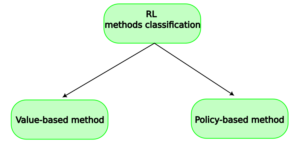
In this method, state-action value function \(Q(s,a)\) is used by the agent to decide which action to take. \(Q(s,a)\) is expected total reward from the current state \(s\) and action \(a\) upto the agent's terminal state

\begin{equation*} a = \arg\max_{a} Q(s,a) \end{equation*} Policy-based method:

In this method, agent take the action directly based on state with the help of policy function which maps state to action.

\begin{equation*} a = f(s) \end{equation*}

Note: RL methods can also be classified in other ways but it easy to understand RL if we prefer to classify it as value-based and policy-based.

Monte-Carlo Policy-Gradient Method (REINFORCE)

Every problem in reinforcement learning is approached with a intention of finding such a policy which can make agent to be able to follow the best possible trajectory. To do so, we need to first set the objective function accordingly: \begin{align} J(\theta) &= \displaystyle \mathop{\mathbb{E}}_{\tau \sim \pi'_\theta}[R(\tau)] \end{align} Here \(R(\tau)\) is total reward gained by the agent over the complete trajectory. To maximize the \(J(\theta)\) , the \(\theta\) need to be updated using gradient ascent approach: \begin{equation*} \theta = \theta + \alpha \nabla_\theta J(\theta) \end{equation*} Now lets focus on solving for \(\nabla_\theta J(\theta)\) \begin{align} \nabla_\theta J(\theta) =& \nabla_\theta \displaystyle \mathop{\mathbb{E}}_{\tau \sim \pi'_{\theta}}[R(\tau)] \label{J_grad} \\ =& \nabla_\theta \int \pi'_\theta(\tau) R(\tau) d\tau \notag \end{align} Here we can not do the integration as \(\pi'_\theta(\tau)\) and \(R(\tau)\) both are unknown to us neither we can do monte-carlo approximation of equation \ref{J_grad} because our equation is not in \(\displaystyle \mathop{\mathbb{E}}\)[] term. It has one extra term which is gradient operator outside of \(\mathop{\mathbb{E}}\)[]. So we need to somehow, shift the gradient operator inside the \(\mathop{\mathbb{E}}\)[] in equation \ref{J_grad}.
\begin{align*} \nabla_\theta J(\theta) =& \nabla_\theta \int \pi'_\theta(\tau) R(\tau) d\tau\\ =& \int \nabla_\theta(\pi'_\theta(\tau)) R(\tau) d\tau \hspace{2em}\because \nabla_\theta\text{ is a linear operator} \end{align*} To transform this integral into \(\mathop{\mathbb{E}}\)[] from, we need atleast one \(\pi'_\theta(\tau)\) with no gradient operation over it in the above equation. \begin{align*} \nabla_\theta J(\theta) =& \int \frac{\pi'_\theta(\tau)}{\pi'_\theta(\tau)} \nabla_\theta(\pi'_\theta(\tau)) R(\tau) d\tau\\ =& \int \pi'_\theta(\tau) \frac{\nabla_\theta(\pi'_\theta(\tau))}{\pi'_\theta(\tau)} R(\tau) d\tau\\ =& \int \pi'_\theta(\tau) \bigg[ \nabla_\theta \log (\pi'_\theta(\tau)) R(\tau) \bigg] d\tau \hspace{2em}\because \nabla_x\log f(x)= \frac{\nabla_x(f(x))}{f(x)}\\ =& \mathop{\mathbb{E}}_{\tau \sim \pi'_{\theta}}[\nabla_\theta \log (\pi'_\theta(\tau)) R(\tau)] \end{align*} Cheers, we did it !!! We finally were able to write \(\nabla_\theta J(\theta)\) in terms of \(\mathop{\mathbb{E}}\)[], now we can do monte-carlo approximation. \begin{equation*} \nabla_\theta J(\theta) \approx \frac{1}{N} \sum_{j=1}^{N} \nabla_\theta \log (\pi'_\theta(\tau_j)) R(\tau_j) \end{equation*} Okay, so we have successfully approximated the integration but we have more work to do. Now we have another problem, \(\pi^{'}_\theta(\tau)\) is not known to us so we can not take gradient of it. Lets replace \(\pi'_\theta(\tau)\) by equation \ref{eq:prob_of_tau} \begin{align*} \nabla_\theta J(\theta) =& \frac{1}{N} \sum_{j=1}^{N} \nabla_\theta \log (\pi'_\theta(\tau_j)) R(\tau_j)\\ =& \frac{1}{N} \sum_{j=1}^{N} \nabla_\theta \big[\log( p(s_{0,j}) \prod_{i=0}^{T-1} \pi_\theta(a_{i,j}|s_{i,j})p(s_{i+1,j}|s_{i,j},a_{i,j}) )\big]R(\tau_j)\\ =& \frac{1}{N} \sum_{j=1}^{N} \nabla_\theta \big[\underbrace{\log( p(s_{0,j}))}_\text{do not depend on \(\theta\)}+\; \log( \prod_{i=0}^{T-1} \pi_\theta(a_{i,j}|s_{i,j}))\;+\;\underbrace{\log(\prod_{i=0}^{T-1} p(s_{i+1,j}|s_{i,j},a_{i,j})}_\text{do not depend on \(\theta\)} )\big]R(\tau_j)\\ =& \frac{1}{N} \sum_{j=1}^{N} \big[\cancelto{0}{\nabla_\theta \log(p(s_{0,j}))}+\; \nabla_\theta\log( \prod_{i=0}^{T-1} \pi_\theta(a_{i,j}|s_{i,j}))\;+\;\cancelto{0}{\nabla_\theta\log(\prod_{i=0}^{T-1} p(s_{i+1,j}|s_{i,j},a_{i,j}) )}\big]R(\tau_j)\\ =& \frac{1}{N} \sum_{j=1}^{N} \big[\nabla_\theta \log(\prod_{i=0}^{T-1} \pi_\theta(a_{i,j}|s_{i,j}))\big]R(\tau_j)\\ =& \frac{1}{N} \sum_{j=1}^{N} \big[\nabla_\theta \sum_{i=0}^{T-1}\log( \pi_\theta(a_{i,j}|s_{i,j}))\big]R(\tau_j)\\ =& \frac{1}{N} \sum_{j=1}^{N} \sum_{i=0}^{T-1}\nabla_\theta\log( \pi_\theta(a_{i,j}|s_{i,j}))R(\tau_j)\\ \end{align*} Now the above equation can be used for updating policy parameter.

Variance reduction technique

REINFORCE idea was originated in 1992 in Ronald J. Williams paper. The algorithm has showed the way to solve the RL problem but has some issue. The updation of policy parameter \(\theta\) is not gradual, it has lot of variance. This makes it difficult for the agent to find the optimum policy. To deal with the issue two effective variance reduction technique can be used.
1) Policy gradient with reward-to-go
2) Policy gradient with baseline

we will understand both the technique intuitively as well as with its mathematical proof.

Lets write the \(\nabla_\theta J(\theta)\) equation in terms of \(\mathop{\mathbb{E}}\)[] (we will need it in this form for mathematical proof in next subsection): \begin{equation} \label{eq:Grad_J_Exp} \nabla_\theta J(\theta) = \mathop{\mathbb{E}}_{\tau \sim \pi'_\theta}\big[ \sum_{i=0}^{T-1}\nabla_\theta\log( \pi_\theta(a_{i}|s_{i}))R(\tau)\big] \end{equation}

1) Policy gradient with reward-to-go

Intuition:

Till now we had used total reward/return in our equation. Now it's time to improve our objective by removing things that are irrelevant to us. Let's think about one thing, what is the motive of agent while it takes a action? Is it to gain more reward in future or is it also to affect the past reward(which is not possible)….. a big NO! So why to keep past reward in our objective function. This is were a new term reward-to-go is introduced which take into the account only the futuristic reward.

Mathematical proof: 

No-Bias proof 

While we try to reduce the variance it is important to keep in mind that this Variance reduction technique should not add any bias in our estimated \(\nabla_\theta J(\theta)\).
\(\textbf{To prove:}\) \begin{equation*} \mathop{\mathbb{E}}_{\tau \sim \pi'_\theta}\big[ \sum_{i=0}^{T-1}\nabla_\theta\log( \pi_\theta(a_{i}|s_{i}))R(\tau)\big] = \mathop{\mathbb{E}}_{\tau \sim \pi'_\theta}\big[ \sum_{i=0}^{T-1}\nabla_\theta\log( \pi_\theta(a_{i}|s_{i}))R_i\big] \end{equation*} \(\textbf{Proof:}\) \begin{align} \mathop{\mathbb{E}}_{\tau \sim \pi'_\theta}\big[ \sum_{i=0}^{T-1}\nabla_\theta\log( \pi_\theta(a_{i}|s_{i}))R(\tau)\big] &= \mathop{\mathbb{E}}_{\tau \sim \pi'_\theta}\big[ \sum_{i=0}^{T-1}\nabla_\theta\log( \pi_\theta(a_{i}|s_{i}))(\sum_{k=0}^{T-1}r(s_k,a_k,s_{k+1}))\big]\notag\\ &= \mathop{\mathbb{E}}_{\tau \sim \pi'_\theta}\big[ \sum_{i=0}^{T-1}\nabla_\theta\log( \pi_\theta(a_{i}|s_{i}))(\sum_{k=0}^{T-1}r(s_k,a_k,s_{k+1}))\big]\notag\\ &= \mathop{\mathbb{E}}_{\tau \sim \pi'_\theta}\big[ \sum_{i=1}^{T-1}\nabla_\theta\log( \pi_\theta(a_{i}|s_{i}))(\sum_{k=0}^{i-1}r(s_k,a_k,s_{k+1}))\notag\\ &\;\;\;\;+ \sum_{i=0}^{T-1}\nabla_\theta\log( \pi_\theta(a_{i}|s_{i}))\underbrace{(\sum_{k=i}^{T-1}r(s_k,a_k,s_{k+1}))}_\text{reward-to-go}\big]\notag\\ &= \mathop{\mathbb{E}}_{\tau \sim \pi'_\theta}\big[ \sum_{i=1}^{T-1}\nabla_\theta\log( \pi_\theta(a_{i}|s_{i}))(\sum_{k=0}^{i-1}r(s_k,a_k,s_{k+1}))\big]\notag\\ &\;\;\;\;+ \mathop{\mathbb{E}}_{\tau \sim \pi'_\theta}\big[\sum_{i=0}^{T-1}\nabla_\theta\log( \pi_\theta(a_{i}|s_{i}))R_i\big] \label{RTG_bias_1}\\ & \hspace{2em}\because\mathop{\mathbb{E}}\text{[ ] is linear operator}\notag \end{align}

Now we need to see whether we can equate the first term from Equation \ref{RTG_bias_1} to zero then our proof would be complete.

\begin{align} \mathop{\mathbb{E}}_{\tau \sim \pi'_\theta}\big[ \sum_{i=1}^{T-1}\nabla_\theta\log( \pi_\theta(a_{i}|s_{i}))(\sum_{k=0}^{i-1}r(s_k,a_k,s_{k+1}))\big] &= \underbrace{\mathop{\mathbb{E}}_{\tau \sim \pi'_\theta}\big[ \sum_{i=1}^{T-1}\nabla_\theta\log( \pi_\theta(a_{i}|s_{i}))\big]}_\text{=0} \notag\\ & \times\mathop{\mathbb{E}}_{\tau \sim \pi'_\theta}\big[(\sum_{k=0}^{i-1}r(s_k,a_k,s_{k+1}))\big] \notag\\ &=0 \hspace{2em}...\text{refer to lemma 1}\label{RTG_bias_2} \end{align}

Action taken based on current state affect state of the agent in future and the reward the agent will get it in future but it does not have any relation with the reward agent has got in the past. So action and the past reward are independent random variable.( \(\mathop{\mathbb{E}}[XY]=\mathop{\mathbb{E}}[X]\mathop{\mathbb{E}}[Y]\) when \(X\) and \(Y\) are independent random variable)
From Equation \ref{RTG_bias_1} and \ref{RTG_bias_2}, it proves that replacing total reward with reward-to-go does not add bias in our estimated \(\nabla_\theta J(\theta)\)

Variance reduction proof 

\(\textbf{To prove:}\) \begin{equation*} Var(\big[ \sum_{i=0}^{T-1}\nabla_\theta\log( \pi_\theta(a_{i}|s_{i}))R(\tau)\big]) > Var(\big[ \sum_{i=0}^{T-1}\nabla_\theta\log( \pi_\theta(a_{i}|s_{i}))R_i\big]) \end{equation*} \(\textbf{Proof:}\) \begin{align} \text{I will write about it in detail very soon whenever I get some time :)} \notag \end{align}

2) Policy gradient with baseline

Intuition:

Baseline helps the agent to know whether the action taken was better than average or below average. Action taken by the agent is average ideally only when the agent starts to explore a similar trajectory every time and this indicates that now there is no need to update the policy.

Mathematical proof:

No-Bias proof 

\(\textbf{To prove:}\) \begin{equation*} \mathop{\mathbb{E}}_{\tau \sim \pi'_\theta}\big[ \sum_{i=0}^{T-1}\nabla_\theta\log( \pi_\theta(a_{i}|s_{i}))(R_i-b)\big] = \mathop{\mathbb{E}}_{\tau \sim \pi'_\theta}\big[ \sum_{i=0}^{T-1}\nabla_\theta\log( \pi_\theta(a_{i}|s_{i}))R_i\big] \end{equation*} \(\textbf{Proof:}\) \begin{align} \mathop{\mathbb{E}}_{\tau \sim \pi'_\theta}\big[ \sum_{i=0}^{T-1}\nabla_\theta\log( \pi_\theta(a_{i}|s_{i}))(R_i-b)\big] &= \mathop{\mathbb{E}}_{\tau \sim \pi'_\theta}\big[ \sum_{i=0}^{T-1}\nabla_\theta\log( \pi_\theta(a_{i}|s_{i}))R_i\big] \notag\\ &\;\;\;-\mathop{\mathbb{E}}_{\tau \sim \pi'_\theta}\big[ \sum_{i=0}^{T-1}\nabla_\theta\log( \pi_\theta(a_{i}|s_{i}))b\big] \label{BL_bias_1}\\ \end{align}

Now we need to show second term from above Equation \ref{BL_bias_1} equal to zero then our proof will be complete. The second term can be written as:

\begin{align} \mathop{\mathbb{E}}_{\tau \sim \pi'_\theta}\big[ \sum_{i=0}^{T-1}\nabla_\theta\log( \pi_\theta(a_{i}|s_{i}))b\big] &= \mathop{\mathbb{E}}_{\tau \sim \pi'_\theta}\big[ \nabla_\theta\log( \pi'_\theta(\tau))b\big] \notag \\ &= \int \pi'_\theta(\tau) \nabla_\theta\log( \pi'_\theta(\tau))bd\tau \notag\\ &= \int \cancel{\pi'_\theta(\tau)} \frac{\nabla_\theta\pi'_\theta(\tau)}{\cancel{\pi'_\theta(\tau)}}bd\tau \notag\\ &= b\nabla_\theta \int \pi'_\theta(\tau)d\tau \notag\\ &= b\nabla_\theta .1 \hspace{2em}\because \int p(x)dx=1\notag\\ &= b \times 0 \notag\\ &= 0 \label{BL_bias_2} \end{align}

From Equation \ref{BL_bias_1} and \ref{BL_bias_2}, it proves that baseline do not add bias in our estimated \(\nabla_\theta J(\theta)\)

Baseline derivation for least variance 

\begin{align*} Var[x]&=\mathop{\mathbb{E}}[x^2] + \mathop{\mathbb{E}}[x]^2\\ \therefore Var\big[ \nabla_\theta\log( \pi_\theta'(\tau))(R(\tau)-b)\big] &= \mathop{\mathbb{E}}_{\tau \sim \pi'_\theta}\big[ (\nabla_\theta\log( \pi_\theta'(\tau))(R(\tau)-b))^2\big] \\ &\hspace{2em}+ \underbrace{\mathop{\mathbb{E}}_{\tau \sim \pi'_\theta}\big[ \nabla_\theta\log( \pi_\theta'(\tau))(R(\tau)-b)\big]^2}_\text{this has no effect as baseline adds no bias}\\ \text{To find best baseline, solve for }& \frac{dVar}{db}=0\text{ and let }f(\tau)=\nabla_\theta\log( \pi_\theta'(\tau))\\ \frac{d}{db}Var\big[ f(\tau)(R(\tau)-b)\big]&= \frac{d}{db}\mathop{\mathbb{E}}_{\tau \sim \pi'_\theta}\big[ (f(\tau)(R(\tau)-b))^2\big]\\ &= \frac{d}{db}(\cancelto{0}{\mathop{\mathbb{E}}_{\tau \sim \pi'_\theta}[f(\tau)^2R(\tau)^2]}-2\mathop{\mathbb{E}}_{\tau \sim \pi'_\theta}[f(\tau)^2R(\tau)b]+b^2\mathop{\mathbb{E}}_{\tau \sim \pi'_\theta}[f(\tau)^2])\\ &= -2\mathop{\mathbb{E}}_{\tau \sim \pi'_\theta}[f(\tau)^2R(\tau)]+2b\mathop{\mathbb{E}}_{\tau \sim \pi'_\theta}[f(\tau)^2])=0\\ \therefore b = \frac{\mathop{\mathbb{E}}_{\tau \sim \pi'_\theta}[f(\tau)^2R(\tau)]}{\mathop{\mathbb{E}}_{\tau \sim \pi'_\theta}[f(\tau)^2])} \end{align*}

Actor-Critic Method

“Give me six hours to chop down a tree and I will spend the first four sharpening the axe.” - Abraham Lincoln

The framework of this method is build on REINFORCE with baseline method. As we have understood about REINFORCE with baseline method earlier our axe is well sharpened and now it will not take much time to understand Actor-Critic method. Agent in reinforcement learning is termed as Actor and along with 'Actor' model we have one more model named 'Critic' model. This Critic model helps the agent to learn the policy smoothly and has few more advantage which we will get to know when we see it's mathematical equation's \(\\[20pt]\)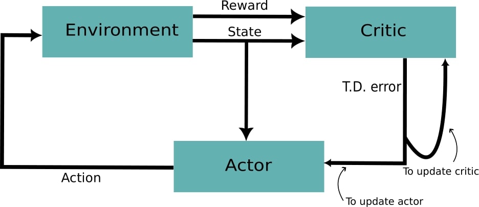
From above figure, we can see that the reward is not directly received by the agent i.e Actor but it is fed into Critic model which gives Temporal Difference (TD) error to the Actor. For now, think T.D. error as some form of modified reward. This TD error is used to update the Actor model i.e it's policy and also it is used to update Critic model. In this algorithm baseline \(b\) is taken as \(V(s_i)\) where \(V(s_i)\) is the expected total reward from state \(s_i\) upto the state \(s_T\). Let's write \(\nabla_\theta J(\theta)\) expression: \begin{align*} \nabla_\theta J(\theta) &= \sum_{j=1}^{N}\sum_{i=0}^{T-1}\nabla_\theta\log( \pi_\theta(a_{i,j}|s_{i,j}))(R_{i,j}-b)\\ &= \sum_{j=1}^{N}\sum_{i=0}^{T-1}\nabla_\theta\log( \pi_\theta(a_{i,j}|s_{i,j}))(R_{i,j}-V(s_{i,j}))\\ \end{align*} Using above equation we can not update the policy at each timestep as we need atleast one complete trajectory to know reward-to-go value. we can sort this out by approximating reward-to-go as follows: \begin{align*} R_i &= r_i + \gamma r_{i+1} + \gamma^2 r_{i+2} + \cdots + \gamma^{T-1} r_{T-1} \hspace{2em}0 \leq \gamma \leq 1\\ &= r_i + \gamma (r_{i+1} + \gamma r_{i+2} + \cdots + \gamma^{T-2} r_{T-1})\\ &= r_i + \gamma R_{i+1} \\ &\approx r_i + \gamma V(s_{i+1}) \end{align*} \(\gamma\) is a discount factor which is used to give geometric weightage to reward at each timestep. Now \(\nabla_\theta J(\theta)\) can be written as: \begin{equation*} \nabla_\theta J(\theta) = \nabla_\theta\log(\pi_\theta(a_{i}|s_{i}))\underbrace{(r_i + \gamma V_\phi(s_{i+1})-V_\phi(s_{i}))}_\text{TD} \end{equation*} This above equation does not need to know the reward across the whole trajectory. Hence, it can be used to update policy at each timestep. The T.D puts a constraint on the updation of policy and has effects as follow: \begin{align*} r_i + \gamma V_\phi(s_{i+1})>V_\phi(s_{i})&\rightarrow\text{update's \(\theta\) in the direction of estimated }\nabla_\theta \log\pi_\theta(a|s)\\ r_i + \gamma V_\phi(s_{i+1})=V_\phi(s_{i})&\rightarrow\text{no update; might have reached optimum solution}\\ r_i + \gamma V_\phi(s_{i+1})< V_\phi(s_{i})&\rightarrow \text{update's \(\theta\) in the opposite direction of estimated }\nabla_\theta \log\pi_\theta(a|s) \end{align*} \(\\[20pt]\)
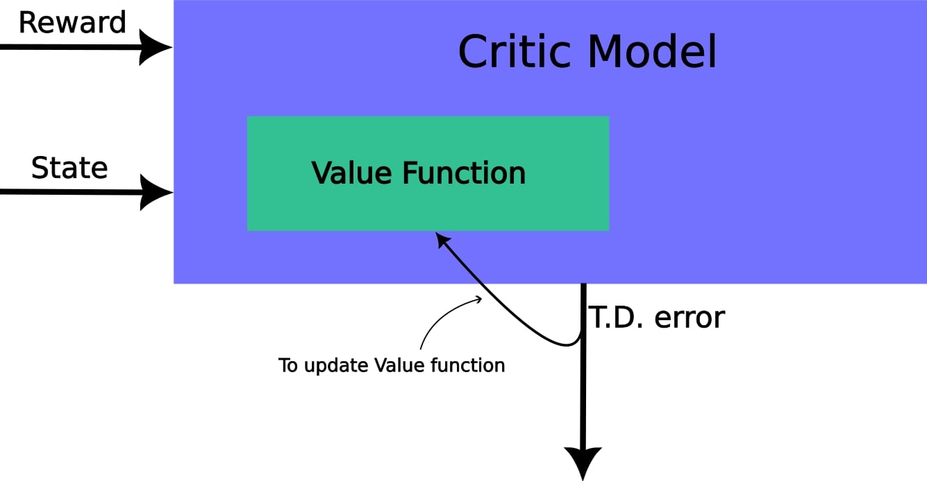
As seen from the above figure when we update Critic model, it is actually the state value function \(V(s)\) that gets updated. Here state value function \(V(s)\) is parameterized by \(\phi\). Its minimization objective function is: \begin{equation*} J(\phi) = r_i + \gamma V_\phi(s_{i+1})-V_\phi(s_{i}) \end{equation*} As the objective is to minimize the T.D error, we will update parameter of state value function by gradient descent approach: \begin{equation*} \phi = \phi - \alpha \nabla_\phi J(\phi) \end{equation*}

Note: I feel it is more appropriate to say just 'temporal difference' when it is feed to Actor model whereas 'temporal difference error' when it is fed into Critic model

---

Algorithm Actor-Critic

---

Initialize parameters \(s\), \(\theta\), \(\phi\), \(\gamma\) and learning rate \(\alpha_\theta\), \(\alpha_\phi\)
for \(t=1...T\)

Sample the action \(a \sim \pi_\theta(s)\)
Sample next state \(s' \sim P(s,a)\) and reward \(r = f(s,a,s')\) from environment
Update:

\(\theta=\theta+\alpha_\theta\nabla_\theta\log(\pi_\theta(a|s))(r+ \gamma V_\phi(s')-V_\phi(s))\)
\(\phi = \phi - \alpha_\phi\nabla_\phi(r+\gamma V_\phi(s')-V_\phi(s))\)

\(\hspace{1.8em}\)set \(\hspace{0.5em}s\leftarrow s'\)
end

---

I hope you had a great time reading this blog. Have a great day ahead !!!

References

1. Sutton, Richard S., and Andrew G. Barto. Reinforcement learning: An introduction. MIT press, 2018.
2. Ravichandiran, Sudharsan. Deep Reinforcement Learning with Python: Master classic RL, deep RL, distributional RL, inverse RL, and more with OpenAI Gym and TensorFlow. Packt Publishing Ltd, 2020.
3. https://danieltakeshi.github.io/2017/03/28/going-deeper-into-reinforcement-learning-fundamentals-of-policy-gradients/
4. https://spinningup.openai.com/en/latest/spinningup/rl_intro.html
5. http://rail.eecs.berkeley.edu/deeprlcourse-fa17/f17docs/lecture_4_policy_gradient.pdf