Why the notation of discrete state-space model is not consistent across literature?

Posted on 3^rd July, 2024

Pre-requisite: Not required

Content:

Introduction
Background
Explaination

Case: 1) when '\(u\)' is external disturbance input
Case: 2) when '\(u\)' is external control input

Introduction

Discrete state-space model(process equation) is mathematically defined as \(x_{k+1}=f(x_k,u_k)\) where '\(k\)' is timestep, '\(x\)' is state of the dynamical system and '\(u\)' is an external input to the dynamical system. In literature there are two versions of process equation: \(x_{k+1}=f(x_k,u_k)\) and \(x_{k+1}=f(x_k,u_{k+1})\) when '\(u\)' is external input. One might get confused and might think which one of them is correct. Lets find out the truth . . .

Background

A closed form solution of discrete state space can be derived if its continuous state-space model is linear w.r.t to '\(x\)'. Let's consider an linear continuous state-space model as shown below: \begin{equation*} \dot{x} = Ax+Bu \end{equation*} Now derivation of discrete state-space model can be done as followed: (for ease of derivation let '\(x\)' be scalar) \begin{align*} \dot{x} & = Ax + Bu \\ \dfrac{dx}{dt} & = Ax + Bu\\ dx & = (Ax + Bu)dt \\ \dfrac{dx}{(Ax + Bu)} & = dt \end{align*} Integrating both sides \begin{align*} \int_{x_k}^{x_{k+1}} \dfrac{1}{(Ax + Bu)}dx & = \int_{t_k}^{t_{k+1}} dt \\ \dfrac{\ln (Ax_{k+1} +Bu_k) - \ln (Ax_k + Bu_k)}{A} &= t_{k+1} - t_k \\ \ln\big(\dfrac{Ax_{k+1} +Bu_k}{Ax_k + Bu_k}\big) &= A \Delta t \\ \dfrac{Ax_{k+1} +Bu_k}{Ax_k + Bu_k} & = \exp (A \Delta t) \\ Ax_{k+1} +Bu_k & = \exp (A \Delta t)(Ax_k + Bu_k) \\ Ax_{k+1} &= A_dAx_k + (A_d-I)Bu_k \\ x_{k+1} &= A^{-1}A_dAx_k+A^{-1}(A_d-I)Bu_k \\ x_{k+1} &= A_dx_k+B_du_k \\ x_{k+1} &= f(x_k,u_k) \end{align*} Here, \(A_d = \exp(A \Delta t)\) and \(B_d=A^{-1}(A_d-I)B\)

why continuous state-space model is called as continuous ?

Continuous state-space model do not have the restriction as of discrete state-space model. A discrete state-space model can be used only to estimate state at specific timestep \(t_{k+1}\) based on state at \(t_k\) so it is called discrete. But it can not tell about the state of the system in between time-interval \(t_k\) and \(t_{k+1}\).
But a Continuous state-space model \(\dot{x}_k=f(x_k,u_k)\) could tell about state at any time. Let the time be \(t_*\) which is close to \(t_k\), then the state at \(t_*\) will be: \begin{align*} x_{t_*} &= x_k + \dot{x}_k(t_* - t_k) \\ &= x_k + f(x_k,u_k)(t_* - t_k) \end{align*}

Explaination

Case: 1) when '\(u\)' is external disturbance input

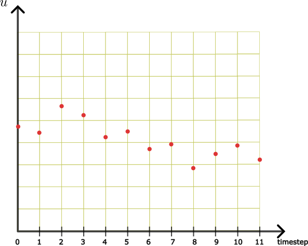
As shown is the above figure, discrete information of external input '\(u\)' to the dynamical system is available because sensors take measurement at discrete time. But in reality '\(u\)' is continuous input, so based on those discrete input throughtout each time-interval some value of input need to be assumed. This is done using one of the two approach as shown in the sub-figures below.

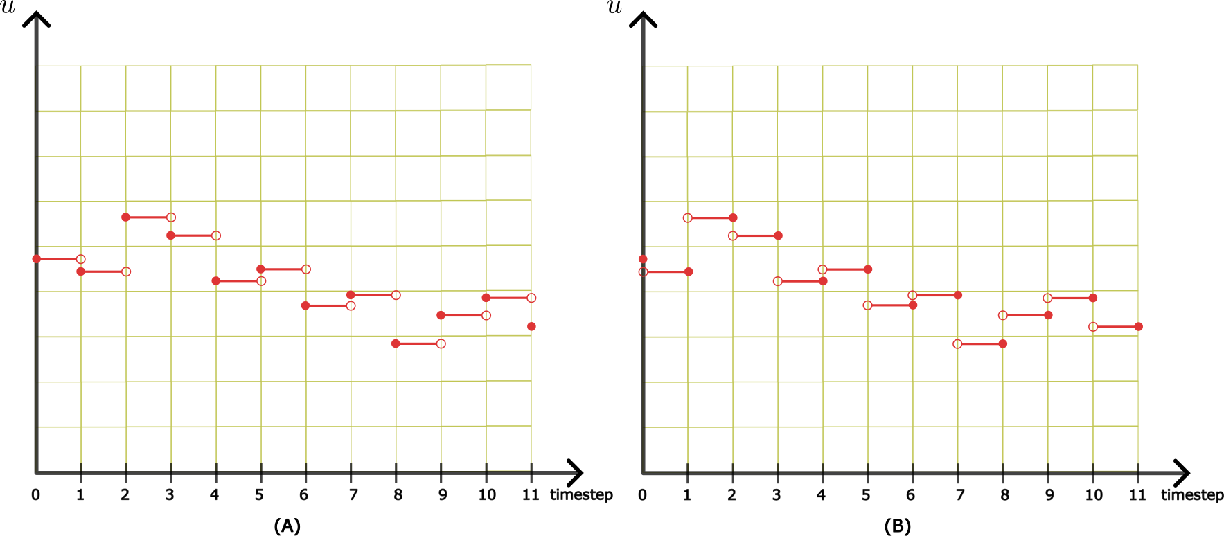
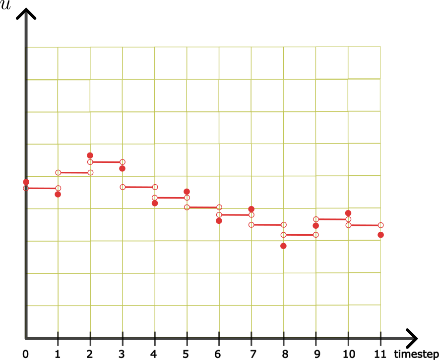
In background section, external input was assumed as per figure (A) in the domain [\(t_k,t_{k+1}\)) and the derivation was carried out. One could also assume external input as per figure (B) in the time domain (\(t_k,t_{k+1}\)] then we would end up with \(x_{k+1}=f(x_k,u_{k+1})\). So in the case of external disturbance input both the versions of discrete state-space model are correct. \begin{equation*} x_{k+1} = f(x_k,u_k) \text{ or } f(x_k,u_{k+1}) \end{equation*}

Can the discrete state-space model be better than the present one's ?

1) A simplest performance wise better alternative for a discrete state-space model when '\(u\)' is external disturbance input would be to consider average of '\(u\)' at timestep \(t_k\) and \(t_{k+1}\): \begin{equation*} x_{k+1}=f(x_k,\dfrac{u_k+u_{k+1}}{2}) \end{equation*}

2) A second alternative approach is to consider linearly varying '\(u\)' between the time-interval [\(t_k,t_{k+1}\)]. Doing so for the case of linear continuous state-space model we would end up with: \begin{equation*} x_{k+1} = A_dx_k+(A^*)^{n-1}Bu_{1,k}+(A^*)^{n-2}Bu_{2,k}+\cdots+Bu_{n,k} \end{equation*} Here, \(A^* = \exp(A \Delta t/n),u_{i,k}=u_k+(i-1)(u_{k+1}-u_k)/n\) where \(n\) is finitely large number.

Case: 2) when '\(u\)' is external control input

In this case, as '\(u\)' is external control input it is known to us throughout the time-interval [\(t_k,t_{k+1}\)] and so there is no assumption needed as in earlier case. A control input value is decided based on the current state of dynamical system and can be mathematically defined as \(u_{k^+}=f(x_k)\) (Note: \(k^+\) means right hand limit).
As decision of control input and measurement of state of dynamical system '\(x\)' is not a simultaneous task, first \(x\) is measured and then control decision is taken. This \(u_{k^+}\) is constantly given to the system until measurement of state of dynamical system is obtained at next timestep \(t_{k+1}\). Hence the control input would follow only the pattern as per figure (B) and we would have discrete state-space model as below: \begin{equation*} x_{k+1} = f(x_k,u_{k+1}) \end{equation*}